When video timing matters, average fps is only the beginning.
A file can tell one timing story through timestamps stored in metadata (for example, presentation timestamps, or PTS). The burned-in timestamp visible in the image can tell another. When those two disagree, you may be looking at drift, cadence changes, freezes/repeats, or edits that you can miss if you only trust a single source.
What you're looking at
- Burned-in timecode (OCR): the time display burned into the video frames, read per frame and reduced to whole-second transitions for comparison.
- Playback timing (PTS): per-frame presentation timestamps from the stream/container (ffprobe
best_effort_timestamp_time, with fallbacks), expressed in seconds. - Declared FPS baseline: a reference line computed as
(frame - anchorFrame) / fpswherefpscomes from ffprobe (r_frame_rateoravg_frame_rate) or a custom value. Useful as a baseline, not proof of true cadence.
Why compare burned-in timecode vs metadata?
Burned-in timecode and stream metadata are both information about timing, and neither should be trusted outright. Burned-in timecode is the time display baked into the recording. Metadata timing includes per-frame playback timestamps (PTS) and multiple "frame rate" values that tools like ffprobe report. Comparing these sources can help characterize playback-timing behavior across a clip.
In real workflows, those can diverge:
- Transcodes and edits can rewrite or rebase timestamps while leaving the visible overlay unchanged.
- Cadence can vary even when average fps looks reasonable.
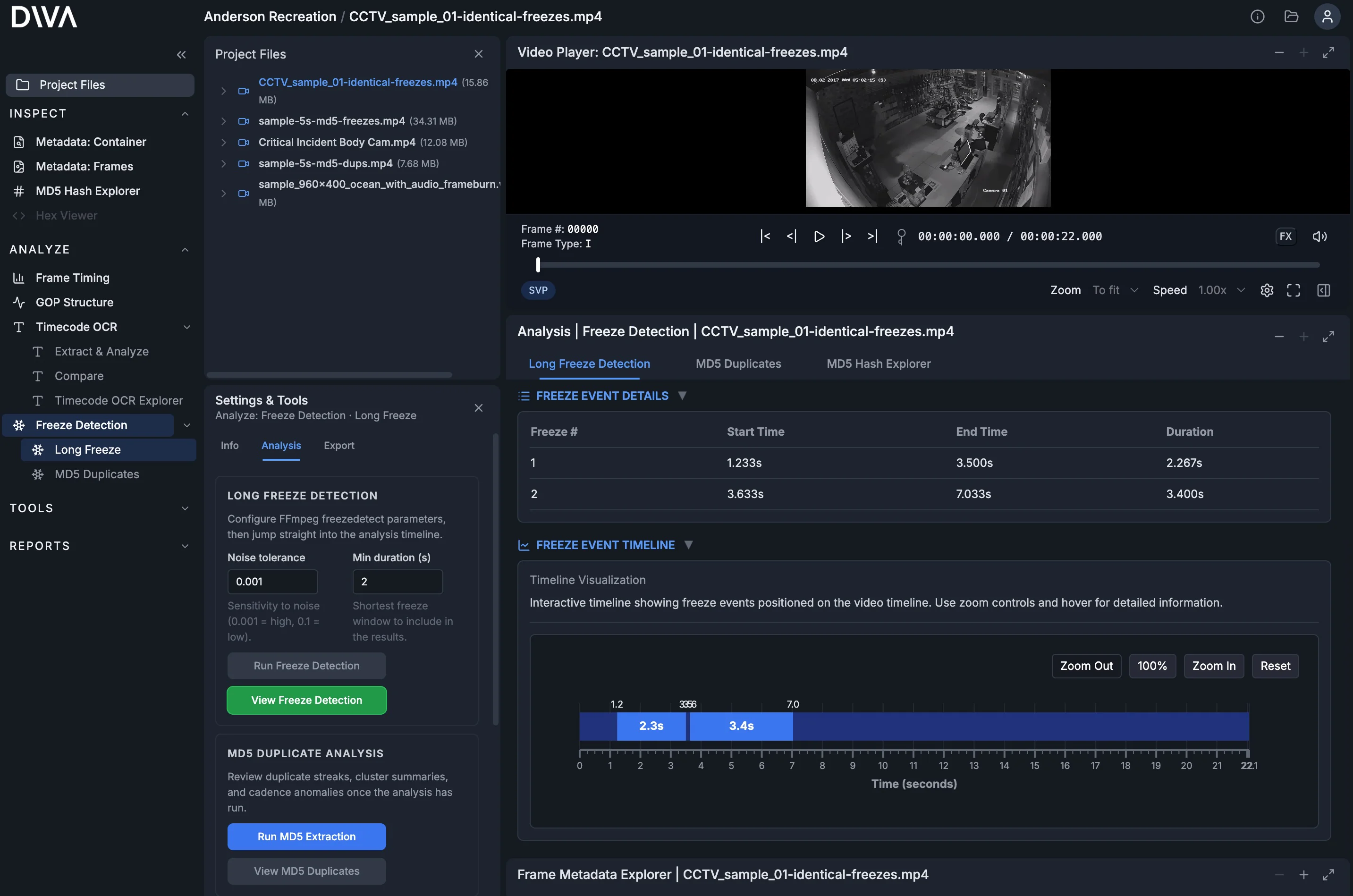
- Freezes/repeats or skipped moments can still produce plausible-looking metadata unless you compare to the burned-in time display.
In this guide, the screenshots focus on a common real-world outcome: cadence drift.
A simple workflow:
Step 1: Define the extraction
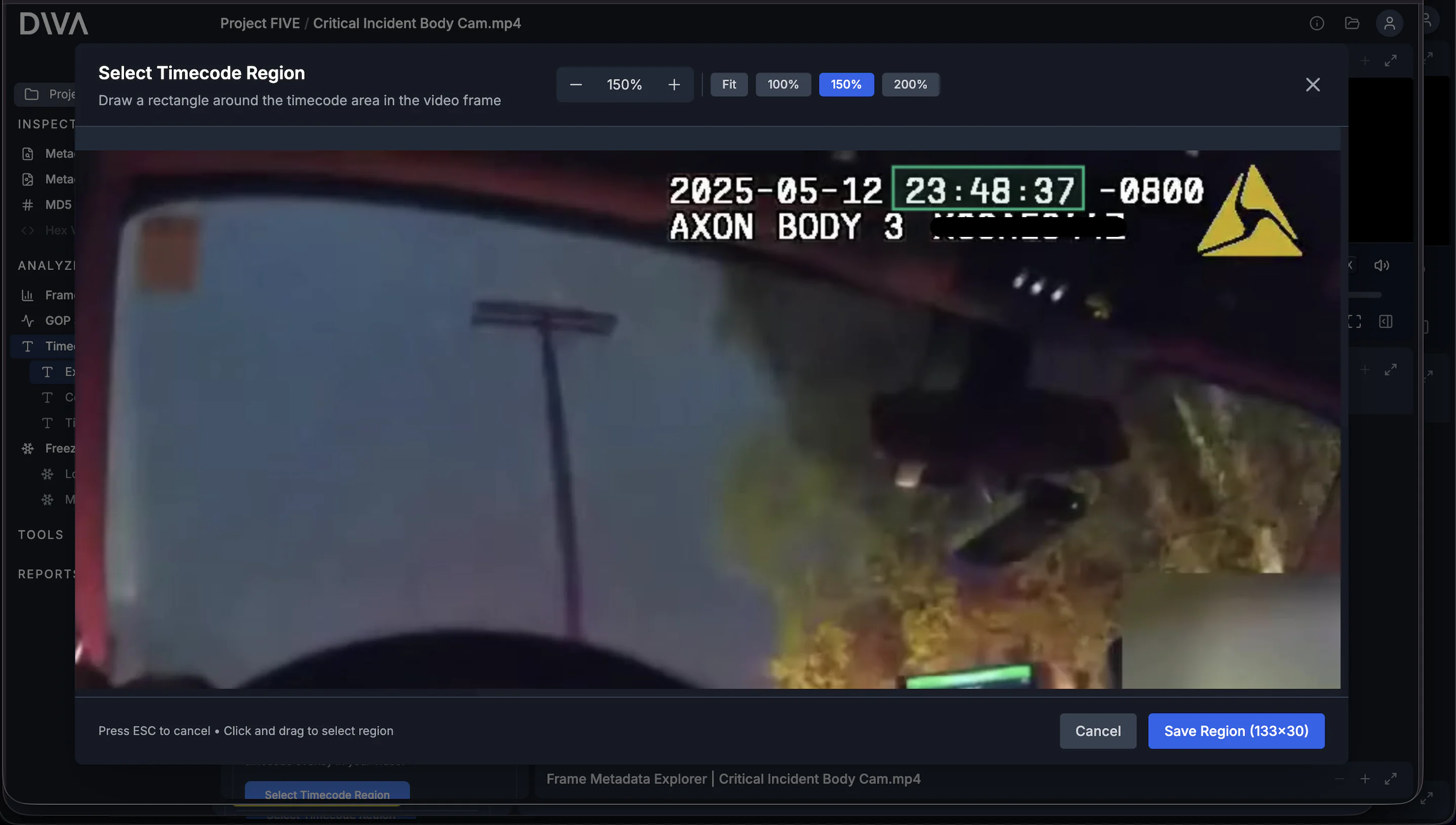
Set the frame range, choose the timecode format, then open the region selector.
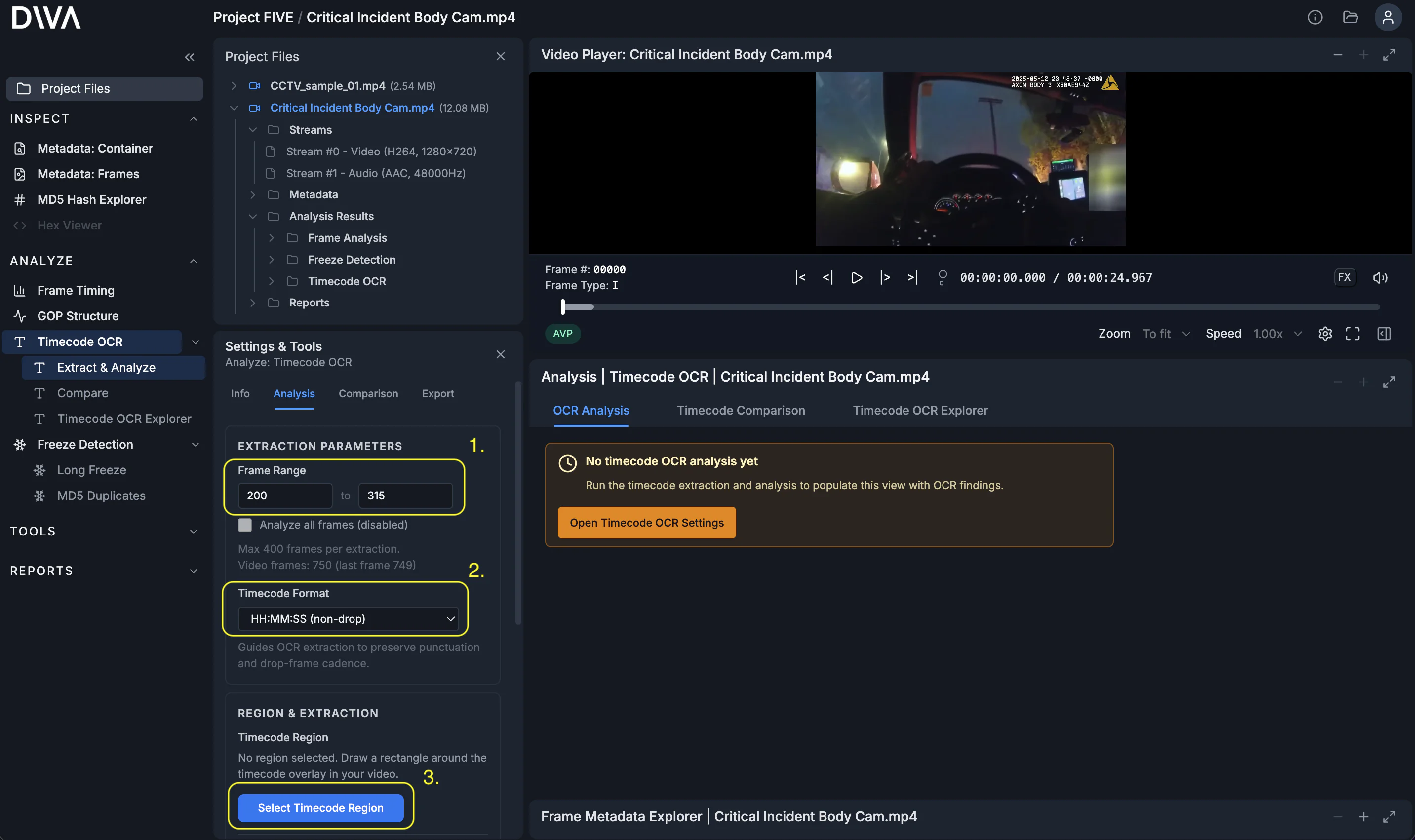
In the region selector modal, draw a rectangle tightly around the on-screen time display. The region matters: it keeps OCR focused on the timestamp area instead of forcing it to interpret the full frame.
Step 2: Extract Timecode OCR
Press Extract Timecode OCR. DIVA extracts the burned-in timestamp into structured data so it can be analyzed consistently and audited. Under the hood, DIVA uses state-of-the-art AI models to read the time display. This approach is more accurate and robust than older OCR methods such as Tesseract.
Step 3: Run timecode analysis
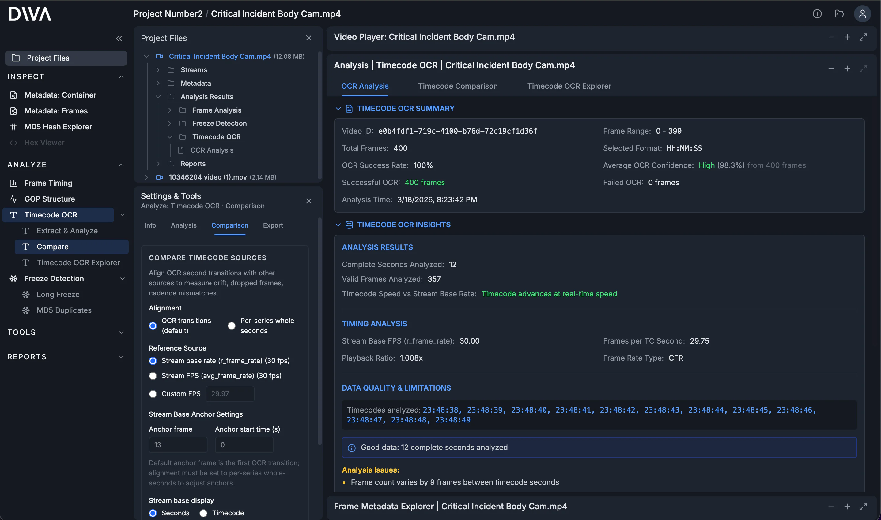
Press Run Timecode Analysis. DIVA compares the observed (OCR) timecode against internal timing sources (including PTS) so timing behavior is easy to inspect and export.
The OCR Analysis summary is your quality check: extraction success/failure counts, confidence summaries, and access to the underlying raw reads. You can review raw outputs and export the data so any chart conclusions are backed by inspectable evidence.
The most important findings (and why they matter)
After analysis, you’ll usually spend time in three views:
- OCR Analysis: extraction quality (success/failure counts, confidence, and raw reads).
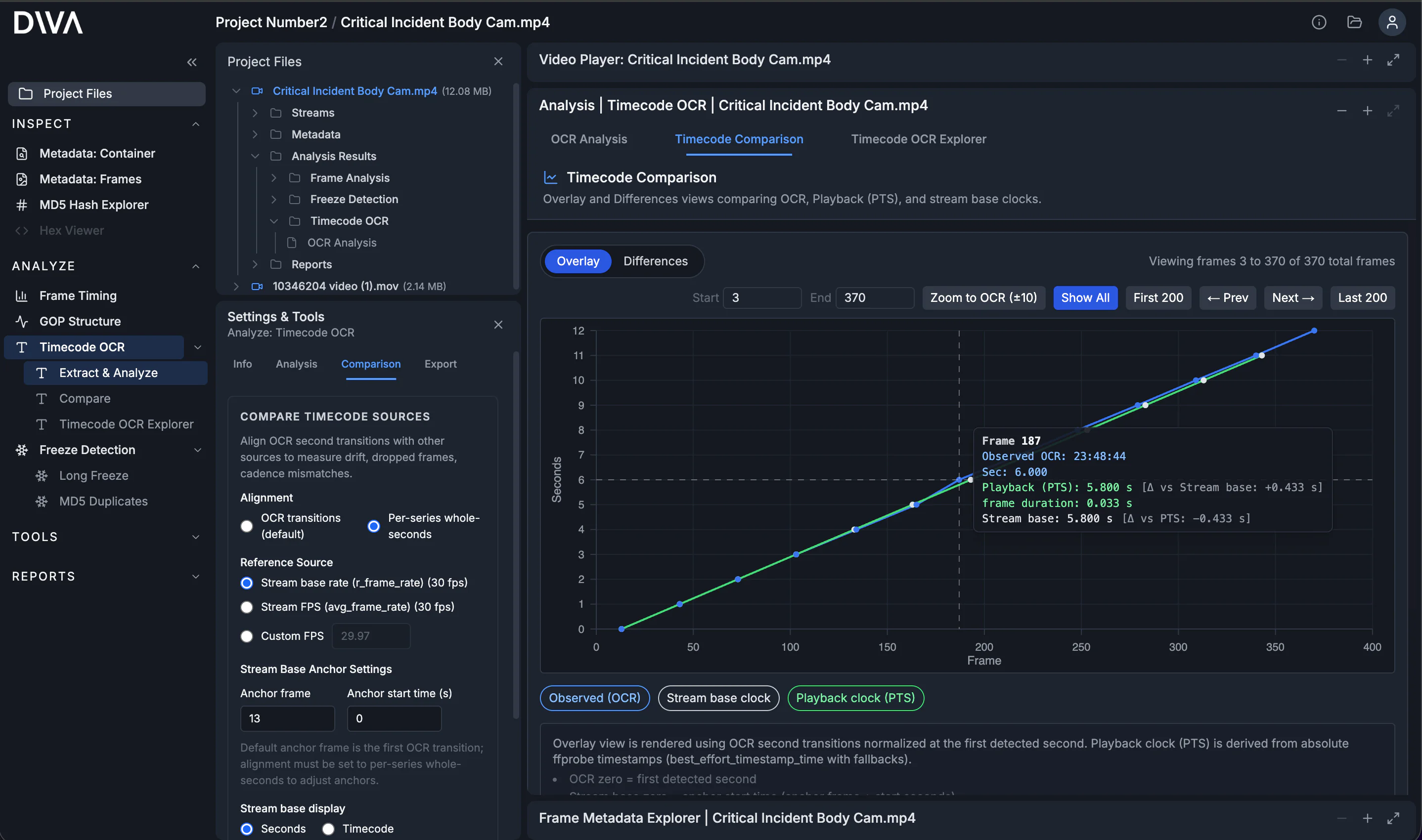
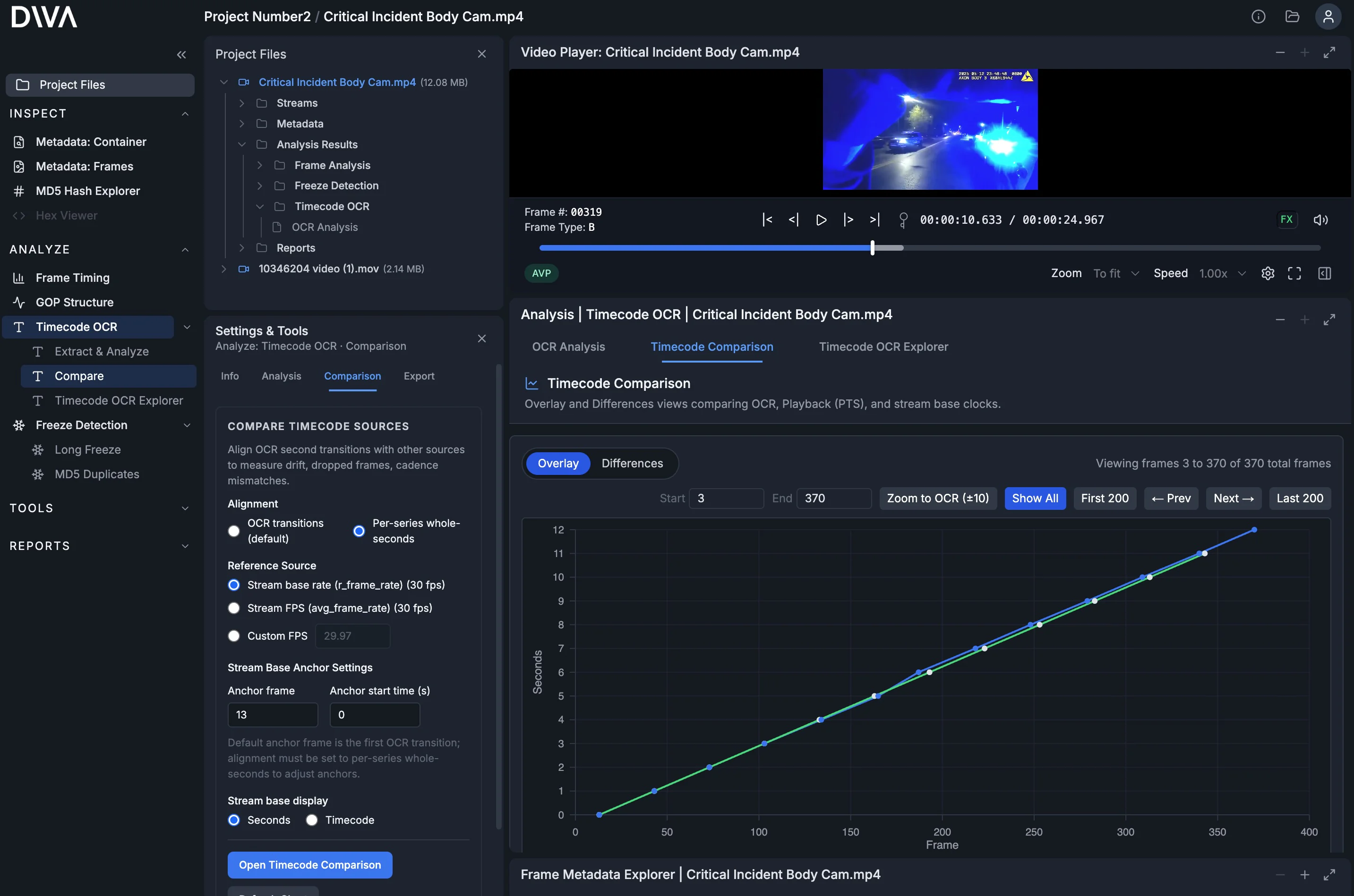
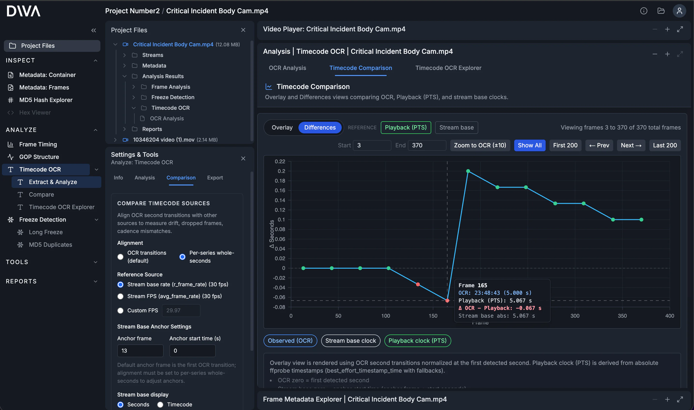
- Timecode Comparison: visual timing alignment across OCR, playback (PTS), and stream timing.
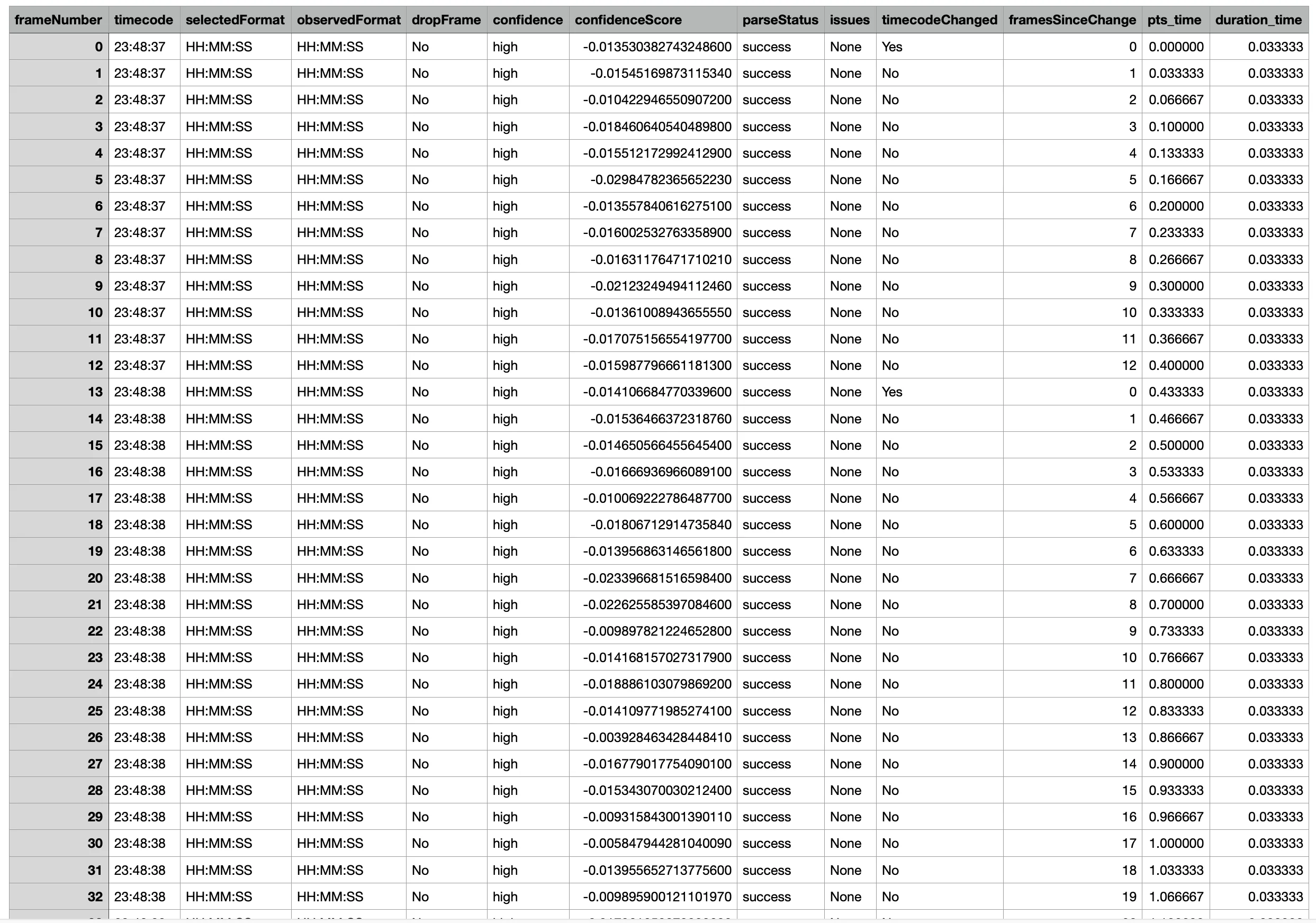
- Timecode OCR Explorer: frame-by-frame table view that makes cadence and second-tick behavior obvious.
What to look for
Here are the highest-signal patterns:
- Mismatch/drift between observed (OCR) time and metadata timing (PTS).
- Cadence inconsistencies, where the number of frames between visible second changes varies unexpectedly.
- Freezes / repeats / jumps in the observed timecode that can indicate duplicated frames, dropped frames, edits, or overlay behavior that isn’t clock-like.
Differences: quantify the mismatch
When you switch to Differences, DIVA plots deltas between series so you can quantify how much (and where) they disagree. For cadence drift, you often see a delta that ramps, steps, or bends instead of staying flat.
Timecode OCR Explorer
The Timecode OCR Explorer is a tabulated view of the OCR results by frame. It includes the extracted time display, confidence in the interpretation of values, and any flagged issues. The table also includes per-frame timing metadata from the file (PTS, and duration when available). It also computes Frames Since Change, which counts how many frames pass for each tick of the second counter in the burned-in time display.
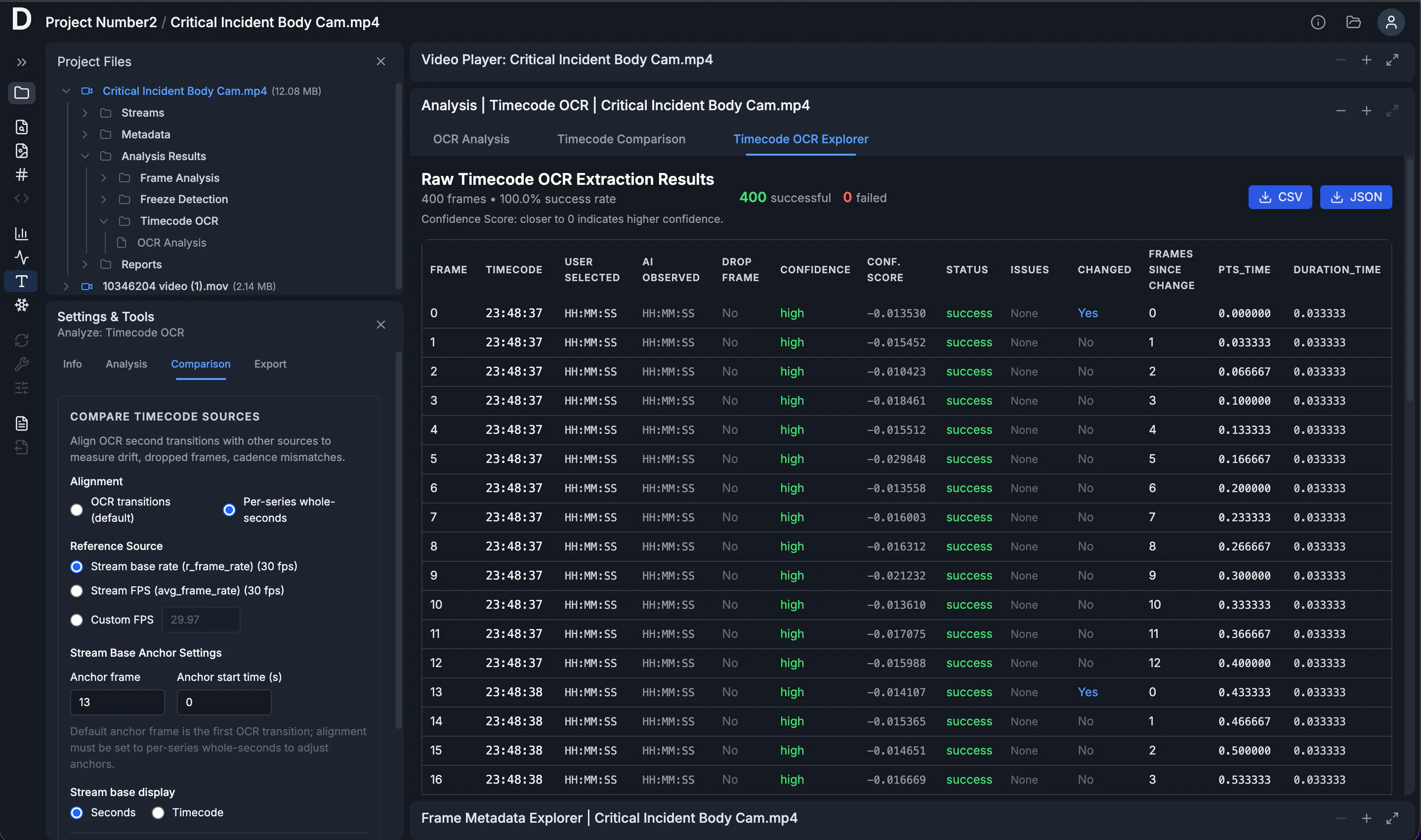
Export the raw rows as CSV/JSON.
Next: go deeper on timing and structure
If you have access to the original recording device, you can sometimes do a controlled reference recording to learn the device's true timing behavior. A common forensic tool is a lightboard reference recording, which gives you a known frame-interval timebase and produces per-frame reference timing data (from the LED pattern). That can complement Timecode OCR by letting you compare the burned-in time display (via OCR) and the file's PTS-derived playback timing against a known reference when you need to separate capture behavior from container/encode/playback behavior.
And when timecode mismatches suggest something more than drift, DIVA includes other push-button analyses that pair well with Timecode OCR:
- Freeze Detection: surface long freezes and repeated content patterns.
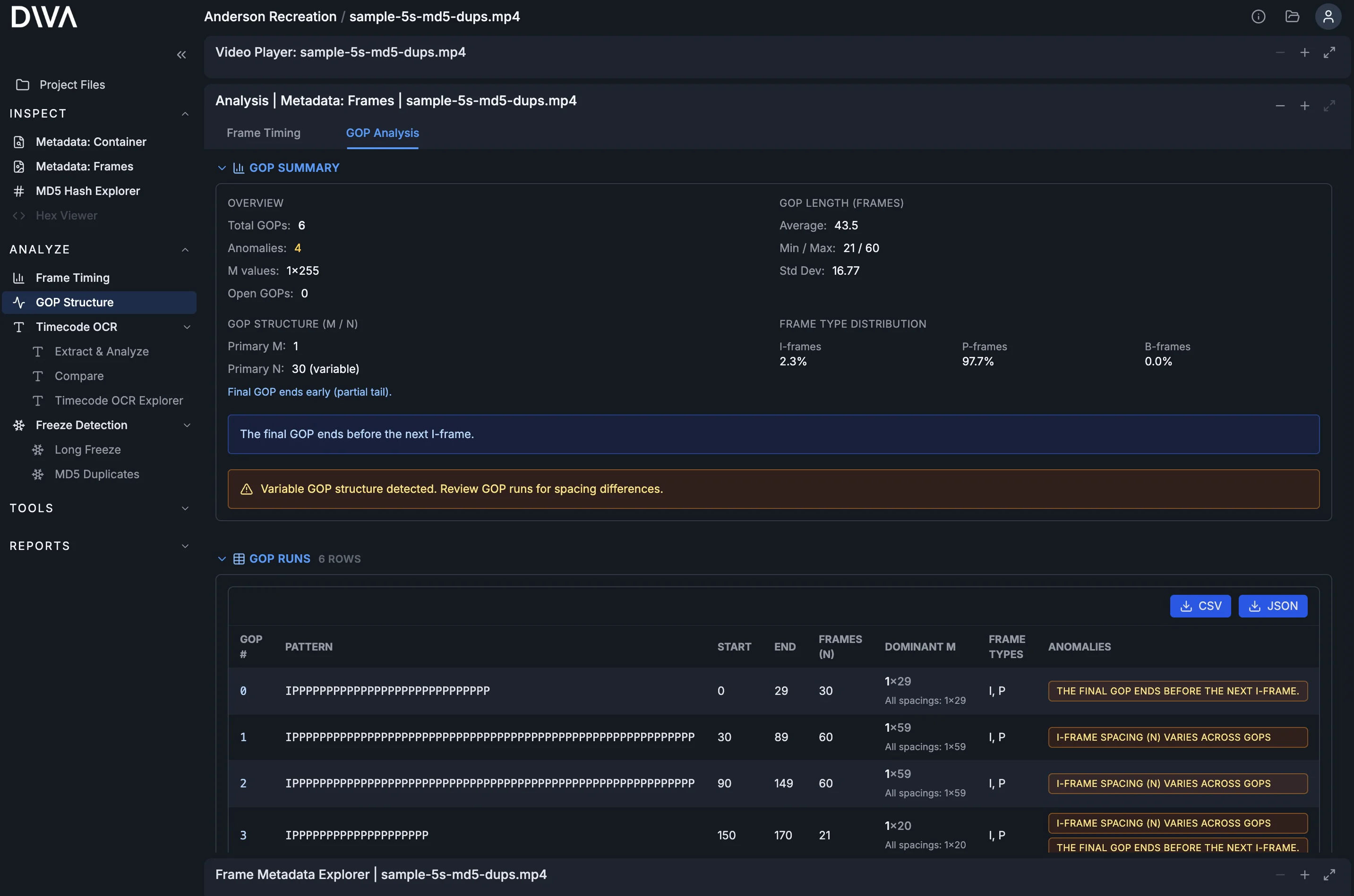
- GOP Structure: inspect keyframe cadence and encoding structure for anomalies that correlate with timing issues.
Closing
This workflow isn’t about blindly trusting “the file” or “the overlay.” It’s about comparing both so timing behavior becomes something you can see, measure, and export.
Timecode OCR Extraction & Analysis follows the same design philosophy as DIVA’s other tools: easy to use, surfaces critical data quickly, and produces exportable results.